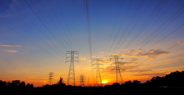
Long Power Transmission Line

ABSTRACT

This continuously changing world demands revolution in everything and even power system comes under it. This caused the power system industry to give in its full potential. The area of quality needs up gradation in long power transmission line. Today’s market is flooded with variety of softwares which can simulate a virtual long power transmission line but when it comes to MATLAB, no one can measure the profile of the voltage as precisely as it can as this is the highlight of the project. The project is aimed at comparing the simulated and practical results. The main focusing of the project is to get deep insight of readings, targets, supplies and a path for simulating the said system in the software. The whole project has two sections. One includes the measurement of the most important and fundamental quantities like Resistance (R), Capacitance (C), Inductance (L) , Voltage (V) and Current (I). The other section requires simulating the coding for MATLAB software. Specifically the former has to be simulated in the latter to find the desired result.

1. INTRODUCTION

Long transmission line is utilized for transferring the power in bulk from the generating station (hydroelectric power plant , thermal power plant etc.) to the substation or substation to the customers. The transmission of power over long distance is typically meted out at 110 KV or 220 KV. It is additionally stepped down to 11 KV or 33 KV by utilizing transformers to distributing centres. Long transmission lines are usually erected by employing conductors, insulators and towers, etc. Conductors used for cables are typically ACSR (aluminum conductor steel reinforced). These conductors have high mechanical strength, low resistance and way better corrosion resistance.

The transmission lines are categorized into three types based on their length. They are:-

1. Short Line: – These lines typically have a range of up to 50 km. In this type of line capacitance and inductance is not taken into account but impedance cannot be ignored.

2. Medium Line: – This length of this line usually falls between 50 and 160 km. In this line, along with impedance, capacitance is also taken into consideration. The methods used to calculate the medium lines are nominal-t method or nominal-π method. When using the nominal- π model, the capacitance is halved both at the sending end and at the receiving end but in nominal-t method the entire proportionate resistance and inductance is a part of this process and is placed at the conclusion of each line.

3. Long Line: – This line is longer than 160 km. This line utilizes distributed parameters for the calculation.

For obtaining the voltage profile, a fictional model of long transmission line is used. The results obtained are then compared with simulated ones. This power line model consists of two conductors 9.6 meters long. These conductors are made up of stainless steel. A megahertz frequency is applied to this line from a frequency generator to make it work like a long transmission line which usually is above 160 km.

2. DESCRIPTION OF RESEARCH

Within the prior stages of the work, writing work has been dine and found the equations for getting the values of resistance, inductance and capacitance by utilizing the predefined dimensions. Also by determining the differential equations we found the voltage equation. Then, the chosen voltage condition is reenacted by one analyst in MATLAB software. After simulation, the estimations are performed and compared with the reenacted ones.

2.1 Long Transmission Line:

Distributed parameters are used instead of lumped parameters for precise calculations in long transmission line. Therefore, the admittance and impedance are uniformly distributed along the line. A diagram below shows a single- phase line of a three-phase network.

     Is                     Ir

      I+dI        I

Gen       Vs       V+dV      V       Vr               Load                                                                                                                                                                                                                                                                                                                                                                                                                                                                                                                                                                                                                                                                                                                                                                                                                                                                                                           dx                                                         x                                                                                                                                                                                                                                                                                                                                                                                                                                                                                                                                                                                                                                                                                                                                                                                                                                                                                                                                                                           Fig 2.1 Schematic diagram of long transmission line.

Representation:

Vs- Sending end Voltage

Vr- Receiving end Voltage

Is- Sending end Current

Ir-Receiving end Current

I= The current at a distance ‘x’

V= the voltage at a distance ‘x’

V+dV=  The voltage at a distance (dx+x)

The impedence in series of the line is Z

Thus,   dV=Izdx

   $\frac{\mathit{dv}}{\mathit{dx}}$

= Iz   (1)

The line admittance is denoted by Y

Thus,  dI=Vydx

   $\frac{\mathit{dI}}{\mathit{dx}}$

= Vy   (2)

Differentiating both the equations with respect to ‘x’

  $\frac{d^{2}V}{d{x}^2}$

= z $\frac{\mathit{dI}}{\mathit{dx}}$

   (3)

And

  $\frac{d^{2}I}{d{x}^2}$

= y $\frac{\mathit{dV}}{\mathit{dx}}$

   (4)

Now, putting the values of $\frac{\mathit{dI}}{\mathit{dx}}$

and $\frac{\mathit{dv}}{\mathit{dx}}$

from (1) and (2) in equations (3) and (4);

   $\frac{d^{2}V}{d{x}^2}$

= yzV   (5)

And

   $\frac{d^{2}I}{d{x}^2}$

= yzI   (6)

Let’s assume the solution of equation (5) to be

 V= A₁ $e^{\sqrt{\mathit{yz} }x}$

+ A₂ $e^{–\sqrt{\mathit{yz}}x}$

  (7)

Again taking the derivative of ‘V’ with respect to ‘x’;

  $\frac{d^{2}V}{d{x}^2}=$

yz(A₁ $e^{\sqrt{\mathit{yz} }x}$

+ A₂ $e^{–\sqrt{\mathit{yz}}x})$

 (8)

Substituting equation (1) in (7);

 I = $\frac{\frac{1}{\sqrt{y}}}{\sqrt{z}}$

A₁ $e^{\sqrt{\mathit{yz} }x}$

– $\frac{\frac{1}{\sqrt{y}}}{\sqrt{z}}$

A₂ $e^{–\sqrt{\mathit{yz}}x}$

 (9)

When x=0, V=Vr and I=Ir;  Substitute these values in equations (7) and (9);

 Vr = A₁+A₂

And

 Ir = $\frac{\frac{1}{\sqrt{y}}}{\sqrt{z}}$

(A₁+A₂)

Put Zc = $\frac{\sqrt{z}}{\sqrt{y}}$

 A₁ = $\frac{\mathit{Vr}+\mathit{IrZc}}{2}$

And

 A₂ = $\frac{\mathit{Vr}–\mathit{IrZc}}{2 }$

Now, put the values of A₁ and A₂ in equations (7) and (9);

And γ = $\sqrt{\mathit{yz}}$

Thus,  V= $\frac{\mathit{Vr}+\mathit{IrZc}}{2}$ $e^{\mathit{\gamma x}}$

+ $\frac{\mathit{Vr}–\mathit{IrZc}}{2 }$ $e^{–\mathit{\gamma x}}$

 (10)

 I = $\frac{\mathit{Vr}/\mathit{Zc}+\mathit{Ir}}{2}$ $e^{\mathit{\gamma x}}$

– $\frac{\mathit{Vr}/\mathit{Zc}–\mathit{Ir}}{2}$ $e^{–\mathit{\gamma x}}$

 (11)

Where Zc= $\frac{\sqrt{z}}{\sqrt{y}}$

and is known as the impedence of the line and γ = $\sqrt{\mathit{yz}}$

is known as the propagation constant

These equations (10) and (11) can also be rewritten using hyperbolic functions. In exponential forms, these can be defined as:

 Sinθ = $\frac{e^{\theta }–e^{–\theta }}{2}$

    (12)

 Cosθ = $\frac{e^{\theta }+e^{–\theta }}{2}$

   (13)

Now, the voltage and current along the line are given by;

 V= Vr coshγx + IrZc sinhγx  (14)

 I= Ir coshγx + $\frac{\mathit{Vr}}{\mathit{Zc}}$

sinhγx  (15)

At the sending end, to obtain voltage and current, let x = l;

Hence, Vs= Vr coshγl + IrZc sinhγl  (16)

 Is= Ir coshγl +  $\frac{\mathit{Vr}}{\mathit{Zc}}$

sinhγl  (17)

Now, replacing Vr and Ir with Vs and Is;

 Vr= Vs coshγl – IsZc sinhγl  (18)

 Ir= Is coshγl – $\frac{\mathit{Vs}}{\mathit{Zc}}$

sinhγl  (19)

When we used these equations before, no load conditions were taken into account. So, at the rreceiving end, the incident and reflected wave are equal.

 Vr= $\mathit{Vs}/\mathit{Cosh\gamma l}$

                                   (20)

2.2 equations for calculating the transmission line parameters

2.2.1 Resistance

 R= $\frac{\mathit{\rho l}}{A}$

Where, ρ= resistivity of the cable,

 l= Length of the cable,

 A= cross-sectional area of the cable.

2.2.2 Inductance

 L= 0.92log $\left(d/r\right)$

*l

Where, r= radius of the cable,

 L= length of the cale,

 d= distance between two cables.

2.2.3 Capacitance

 C= $\left(\frac{0.0121}{\mathit{log}\left(d/r\right)}\right)$

*l

Where, r= radius of the cable,

 l= length of the cable,

 d= distance between two cables.

2.2.4 Frequency

Frequency is given by the formula:

F=v/λ

Also, v= $\frac{1}{\sqrt{\mathit{LC}}}$

 λ=wavelength

λ= 2*l=2*9.6= 19.2

V= 2.92* ${10}^8\raisebox{1ex}{$m$}\!\left/ \!\raisebox{-1ex}{$s$}\right.$

F=15.02 MHz

2.2.5 Shunt Admittance

Y=j2πfc

Y= j6.52* ${10}^{–4}\raisebox{1ex}{$\mathrm{\Omega }$}\!\left/ \!\raisebox{-1ex}{$m$}\right.$

2.2.6 Series Impedence

Z=R+j2 πfc

Z=1.97+j168* ${10}^2\raisebox{1ex}{$\mathrm{\Omega }$}\!\left/ \!\raisebox{-1ex}{$m$}\right.$

2.2.7 Characteristic Impedence

Zc= $\frac{\sqrt{z}}{\sqrt{y}}$

Zc = 520.1-j3.50 $\raisebox{1ex}{$\mathrm{\Omega }$}\!\left/ \!\raisebox{-1ex}{$m$}\right.$

It can be rewritten in r as

R= $\sqrt{\mathit{ZY}}$

R= 0.0022+j0.324 $\raisebox{1ex}{$\mathrm{\Omega }$}\!\left/ \!\raisebox{-1ex}{$m$}\right.$

The above equations are used to find the values of Resistance, Capacitance and Inductance for long power transmission lines. By putting the values of line dimensions in these equations, the researchers found the values of R, L and C to be;

 R= 1.9847Ω

            C=6.8* ${10}^{–7}$

f/m

 L=1.72* ${10}^{–6}$

H/m

3. SYSTEM DESIGN

This project is based upon two transmission line model which are made up of stainless steel. Stainless steel has certain properties. Some of which are described below:

1. Its resistivity is 6.9* ${10}^{–7}$

   .

2. It has high resistance to corrosion.
3. It has more attractive appearance and a higher hot strength.

    3.1 Schematic diagram of long transmission line.

Length of line (9.6m)

                      Sending end          Distance between 2 lines                     Receiving end

Fig 3.1 Model of Long transmission line

The length of the line used in the model is 9.6 meter and the distance between both of them is 5.8 cm. Both the lines are connected from receiving end and sending end and both have the same length. The diameter of the cable is 2.07 mm. A high frequency source is used to make the line work like a line above 160 km of length and measurements are performed. Various equipments used to perform the test are Cathode Ray Oscilloscope (CRO), Frequency Generator and test probe, etc. The software used for simulation is MATLAB 2014b. These devices are described in the section below.

4. DESCRIPTION OF HARDWARE AND SOFTWARE.

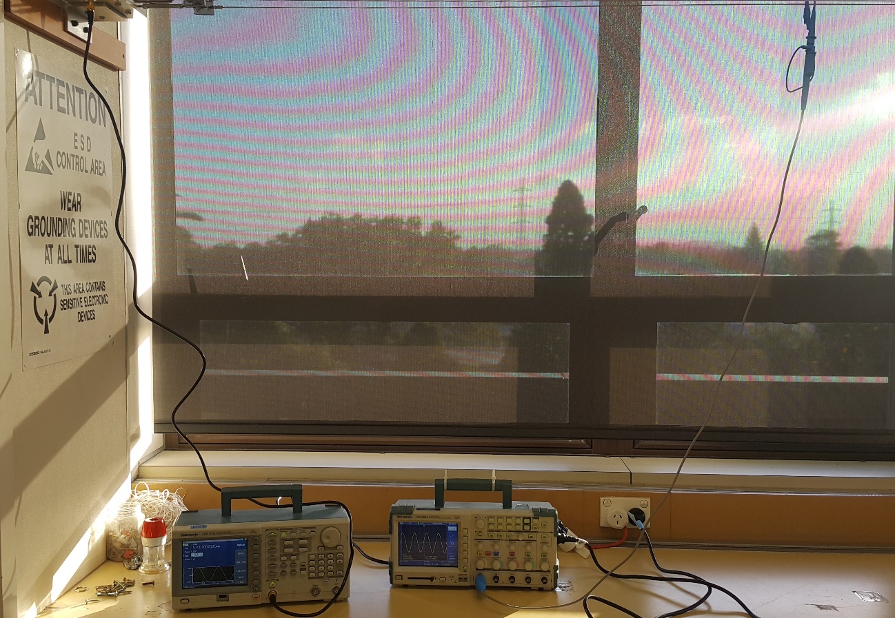
Fig. 4.1 Physical Conection.

            For line measurement, the devices used were:

4.1   Frequency Generator (Tektronix, AFG 3101)

4.2   Oscilloscope (Tektronix, TPS 2014)

4.3   Test Probe

MATLAB software version:

4.4   MATLAB 2014b

4.1 Frequency Generator:

It is mainly a device used to produce waveforms of different frequencies. It includes sine wave, square wave, triangular wave and sawtooth type wave. The particular device used for the project is Tektronix AFG 3101 and it can create frequencies in the range of 1 MHz to 25 MHz. but the project requires only 15 MHz. A clicked picture of frequency generator is shown below.

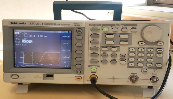
Fig. 4.2 Frequency Generator.

4.2 Oscilloscope:

It is a test instrument that will graphically shows the varying voltage signal. It can also analyze and even show the waveform of a particularly measured value. It cal also convert analog to digital signals. The project uses Tektronix TPS 2014. It has four channels, 100 MHz bandwidth, a long battery life and digital storage. A still of the same is shown below.

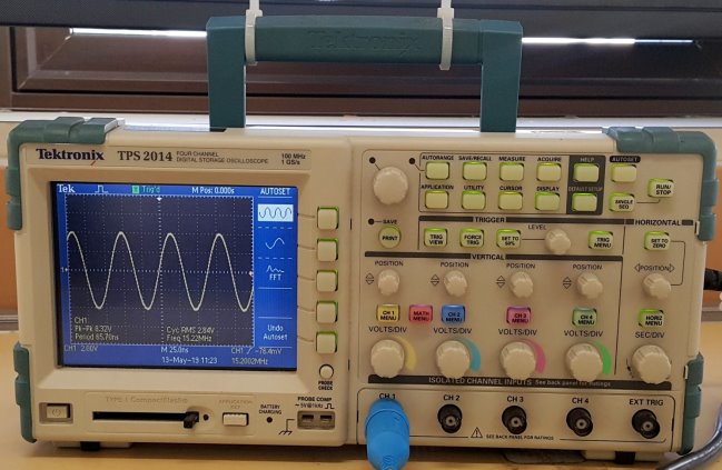
Fig 4.3 Oscilloscope.

4.3 Test probe:

There are various probes available in the market including temperature probe, current probe, etc. In the project, the probe used is voltage probe 1000 v CAT II for the measurement of values along the power cable. A clicked version is shown below.

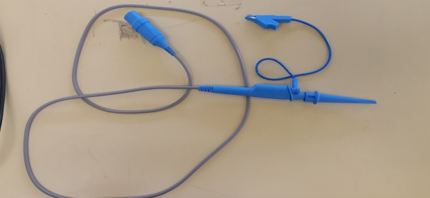
Fig. 4.4 Voltage Probe.

4.4  MATLAB Software:

It is basically used for technical computing. It is developed by Mathworks and is also known as Matrix Laboratory. For the easiness, the researcher has used MATLAB 2014b software for simulating the transmission line model and it is also known as 4^th generation language.

5. MEASUREMENTS

5.1 Practical Measurements

For taking measurements, connect the frequency generator and oscilloscope to 230 volts mains supply. A required frequency is set in the frequency generator. Now, measure the voltage at different distances. Measurements are taken from sending end to receiving end at 0.6 m apart till 9.6 m. the measurements taken are shown in the table below:

Table 1 Calculated Values.

After getting these values, a graph is plotted and this graph is then compared with the one in MATLAB software.

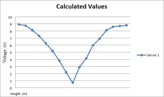
Fig. 5.1 Practical Graph.

By comparing both the practical and simulated one, it is clear that both the graphs look the same.

By looking into the graph, it is clear that the in the simulated one, the voltage drops to zero but in real life thus does not happen. This happens because of impedance in the air which has an impact on practical measurement. Thus, the load impedance is finite.

But in case of simulated one it is vice versa.

5.2 Flow Chart:

Long Transmission Line

MATLAB Simulation               Practical Values

                     Graph of Simulated Values    Graph of calculated values

Comparing graphs of

simulated and calculated

            values

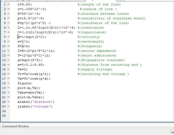
5.3 MATLAB Coding:

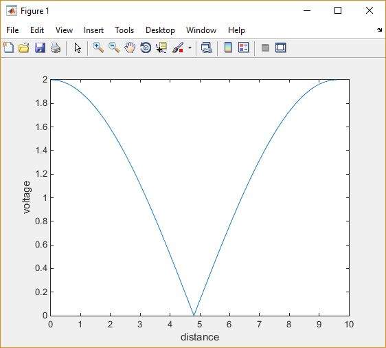
5.4 MATLAB Graph:

COMPARISON:

The researcher analyzes that both the calculated as well as MATLAB simulated graphs are almost the same.

As seen in the simulated one, the researcher assumes that the voltage drops to zero volts but in practicality this does not happen. This happens because of the impedance of the air. As a result, the load impedance is finite. It is also noted that from receiving end to sending end some voltage is present. This has an effect due to which voltage does not drop to zero. But simulated graph shows the absolute value and hence shows near zero volts in between.

CONCLUSION:

To conclude with, it can be said that both the graphs show similar behavior and exhibit same form for long transmission line. The fundamental values have been calculated by employing respective equations and formulas. The calculated value graph does not drop to zero on reaching half the value because of the impedance if the air. To sum up with, the researchers analyze that the behavior of long transmission line in practical and simulated one will be different.

APPENDIX:

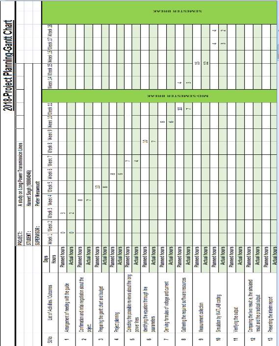
GANT CHART:

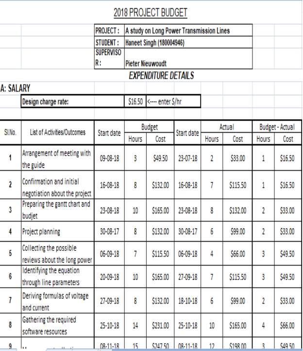
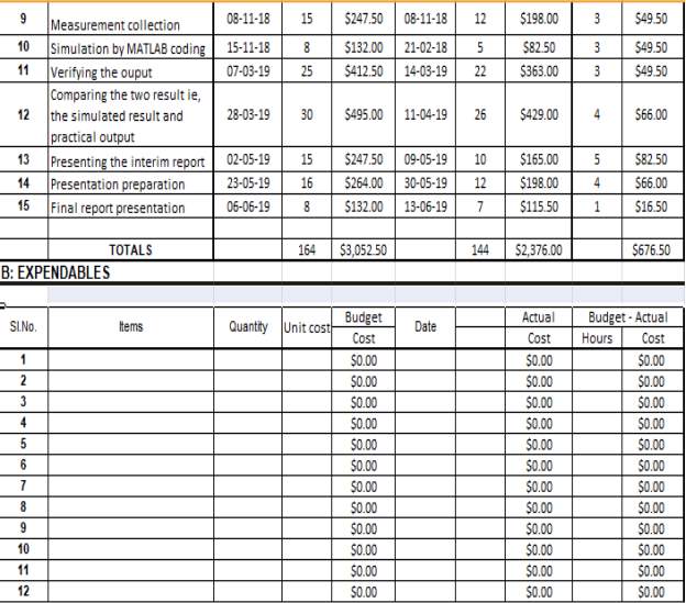
BUDGET CHART:

REFERENCES:

1)     https://en.wikipedia.org/wiki/Function_generator

2)     https://en.wikipedia.org/wiki/Oscilloscope

3)     https://en.wikipedia.org/wiki/Test_probe

4)     https://www.electrical4u.com/long-transmission-line/

5)     https://en.wikipedia.org/wiki/Transmission_line

6)     https://www.google.com/search?q=long+transmission+line+photos&tbm=isch&source=iu&ictx=1&fir=0qktQcxMoCaSgM%253A%252C1zM_zNqegceypM%252C_&vet=1&usg=AI4_-kRJsjekc_gj6ppDj7buHTAiRDu9yQ&sa=X&ved=2ahUKEwiSzM3Q49viAhVz8HMBHcmFAbkQ9QEwBHoECAAQDA&cshid=1560062126783406#imgrc=0qktQcxMoCaSgM:&vet=1

7)     https://www.google.com/search?q=long+transmission+line+photos&tbm=isch&source=lnt&tbs=sur:fmc&sa=X&ved=0ahUKEwiKi8vh9d7iAhXVbn0KHeoIDukQpwUIIw&biw=1366&bih=661&dpr=1#imgrc=zmXme_E8BLfclM: