Landscape Metric Analysis Toll Development
| ✅ Paper Type: Free Essay | ✅ Subject: Environment |
| ✅ Wordcount: 4166 words | ✅ Published: 23 Sep 2019 |
Thesis Proposal
A new tool for Landscape Metric Analysis
Introduction
Landscape metrics measure the composition and configuration of habitats within the Landscape fragments. They are usually dynamic systems and they are affected by intensive human effects or some anthropological changes and eventually, they are altered over time.
This alteration might be a barrier to the landscape structure and changes or might be a cause for the progress of a new type of a habitat, needs to be measured to know more about the changes and the factors causing these changes to the landscape.
To define landscape ecology as a whole, we can say that it studies the internal dynamics and interaction of landscapes. The focus relies mainly on the spatial relationship of landscape elements and ecosystems, functional and structural features of the land mosaic and change that has emerged over time (Dramstad et al. 1995). Landscape ecology accentuates the interaction between spatial pattern and ecological process, that is, the causes and consequences of spatial heterogeneity across a range of scales (Turner et al. 2001). The discipline of Landscape Ecology is emerging as a driving force, both in the domain of theoretical ecology and in applied fields (Sanderson and Harris 2000).
Landscape metrics are the primary tools to understand landscape structure and changes. We use metrics – numeric data relating to the landscape pattern, through these tools. The input to these tools calculating the metrics can be from satellites or maps developed for a specific application through some GIS software, for example, ArcGIS. The input provided to the tool should be of a raster format file or a.TIF file type. Tools like “FRAGSTATS” support a wide variety of input formats to be used with their tool. Landscape metrics allow us to do an objective review of landscape structure.
Literature Review:
In the literature review, we will go through the metrics that are used in the landscape ecology analysis from FRAGSTAT and other tools like LecoS etcetera that has made quantifying landscape metrics possible. Also, we will go through a review of these tools and then further explain the features they offer with respect to landscape metrics. The newly proposed tool for landscape metrics is inspired by “FRAGSTATS” although the tool would address some of the issues present with FRAGSTATS and also provide additional features and ease of using it as a plug-in with a popular GIS software. Fragstats has released the newer version of the tool 4.0. They were originally developed before 1982 and has evolved to version 4.0 covering gradient landscape metrics as well (McGarigal and Marks 1995). Landscape ecology is about focusing on spatial patterns of the landscape elements which calls for these tools to quantitatively analyze and provide with metrics for computation and analysis. They are founded on patterns of environment that influence the ecological patterns. The pattern of the ecological system can be considered to be a fractal that needs to be analyzed as to how it directly or indirectly influences or corresponds to habitats.
The habitats are in which the organisms live, for example are structured spatially at a number of scales. These patterns interact with the organism awareness and conduct to drive a higher level of the process of population dynamics and behavior. If there is any kind of disturbance in the landscape pattern interfere with the maintenance of biodiversity of the habitat and ecological health.
Therefore, the idea of quantifying landscapes came to be of much importance in learning the pattern-process relationships (O’Neill et al. 1988, Turner 1990, Turner and Gardner 1991, Baker and Cai 1992, McGarigal and Marks 1995). This kind of pattern-based study has already resulted in a lot of indices for the landscape analysis patterns. These pattern-based development study has been made possible with the advent of GIS technologies.
There are many different interpretations of the term “landscape” itself. The landscapes usually include an area of land with a mosaic of patches or landscape elements. As per Formal and Gordon (1986) defines landscape as a cluster of interacting ecosystems repeated in a similar pattern throughout the landscape area that is a part of the landscape ecology.
An example of the landscape pattern which is relevant to the area of the study can be considered could be a wildlife habitat, we can see the landscape as a mosaic of habitat patches. These habitat patches could be studied with respect to an organism’s perspective and the scaling of the environment (Forman and Godron,1986).
These habitat patches can be defined with respect to an organism’s perspective and these landscape sizes would differ as well based on the organism under study. These landscapes occupy some spatial scale. The size of the habitat landscape cannot be defined in a particular fashion. Since the size of the landscapes varies with respect to the organisms, we can’t have any definite definition of the size of the landscape.
The landscape pattern can be classified in different ways depending on the data that is collected, and the objectives of the types of data collection, there can be four types of spatial data as per (McGarigal and Marks, 1995). The four types of landscape patterns are defined below:
1. Spatial point patterns:
These point patterns represent a group of units where the geographical locations are of primary interest rather than a quantitative or qualitative attribute of the entity. Such kind of spatial point data analysis are more clustered than expected by chance to find the spatial scale where it is more or less clustered than expected by chance (Dale 1999, Greig-smith 1983)

2. Linear network patterns:
As the name suggests, this is a network of landscape elements which intersect to form a network. An example of this kind of network patterns is a map of streams wherein the data consists of nodes or linkages. With respect to the point patterns, the geographic location, nodes, and corridors are the primary area of interest. The whole goal of the linear network pattern analysis is that they are used to describe the physical structure (e.g., corridor density, mesh size, network connectivity, and circuitry) of the network and there has been a variety of metrics developed for the purpose (Forman 1995, McGarigal and Marks, 1995).
3. Surface patterns:
These are quantitative measurements which vary continuously across the landscape without any explicit boundaries making the data look like representing a three-dimensional surface where the value measured at a geographic surface is represented as a height of the surface. Here we look at the sample and figure out how close they are together and how they are arranged closely with other with respect to the measured variable (McGarigal and Marks, 1995).
4. Categorical map patterns:
Here in this kind of landscape pattern, the data is represented as a mosaic of discrete patches representing a relatively discrete area of relatively homogeneous environmental conditions at a particular scale. These patch boundaries are shown and distinguished by discontinuities in environmental character from surroundings that are relevant to the ecological phenomenon under consideration (Wiens 1976, Kotliar and Wiens 1990).
There are certain metrics that are important in the study of the metrics for landscape analysis and the data available. Patch level metrics form the basic building blocks for categorical maps.
Cell level metrics
There can be cell-level metrics which can be defined for individual cells. They can be used to characterize the neighborhood of each of the cell without any regard for a patch or class affiliation. An example can be an individual organism dispersing from natural habitat to a neighborhood defined by a dispersal distance (McGarigal and Marks, 1995). This would make the typical output to consist of a vector of cell-based measurements in tabular form along with a raster file which will give us an interpretation of the values in the tabulation. The cell metrics can be used for computing for each of the cells in the landscape and the output for the same would consist of a continuous surface grid or map.
Patch level metrics
After cell level, we can have a patch level metrics that would characterize the context of patches. Patch level metrics are very helpful in giving important information in landscape level investigations. Some of the species are affected by edges and are closely associated with patch interiors. This helps in the comparative study of the neighborhood patch that is available which actually helps in understanding the patch and degree of contrast between the patch and the neighborhood (Robbins et al. 1989). The usefulness of this information will depend on the investigation objectives.
Class level metrics
After the cell and patch level metrics, there is a class-level metrics. These class-level metrics are combined over all the patches of a specific type. This would help in finding the greater contribution of large patches to the overall index. An example of this would be a habitat fragmentation (Martin 1992). A habitat fragmentation is a landscape level process. Here in class level metrics, it is divided into smaller habitat fragments. This usually involves a change in landscape composition structure and functions
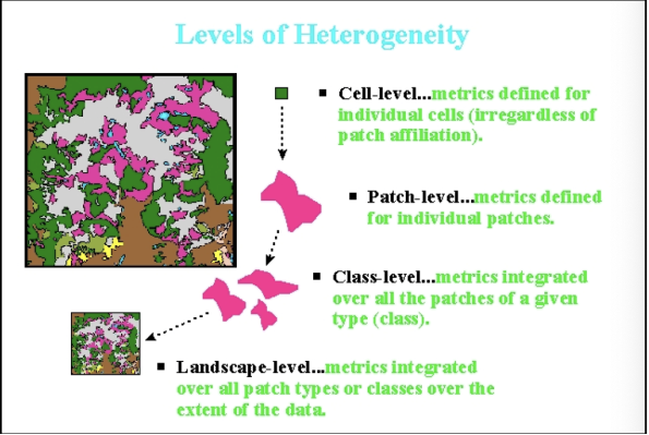
Landscape-level metrics
The next level of metrics in the hierarchy would be landscape level metrics. These might be aggregated into a weighted average or may reflect on aggregate properties of patch mosaic. This quantification of landscape diversity assumed a role in the major focus of landscape ecology. These landscape-level metrics might provide with similar or redundant information with different natural algorithms.
Landscape-level metrics represent the amount and spatial distribution of a single patch which can be considered as a fragmentation index. This makes it important to know what kind of metric we are dealing with even though all of them are related (patch, class, and landscape) (O’Neill et al. 1988, Li 1990, Turner 1990, Turner and Gardner 1991).
As per the hierarchy of the landscape patterns, the next item is to figure about the composition of these landscape patterns. These compositions can be quantified, and they are related to variety and types of the metrics. The diversity indices can be used to summarize the species under study in landscape ecology. There are some measures used to find the composition and they are as follows:
Proportional Abundances
Proportional Abundances of each of the classes that can be derived is the proportion of each class relative to the entire map (McGarigal and Marks, 1995)
Richness
Richness is the number of different patch types. Indices like the Shannon diversity indices are used to calculate the richness in landscape ecology (McGarigal and Marks, 1995).
Evenness
Evenness index is a relative measurement, and this will help in knowing the presence of different patch types. Evenness is usually expressed as a function of maximum diversity possible for a given richness (McGarigal and Marks, 1995).
Diversity
Diversity can be used to measure the richness and evenness that can be computed which depends on the emphasis placed on these components.
Spatial pattern is much more difficult to quantify and refers to the spatial character and arrangement, position, or orientation of patches within the class or landscape. Some aspects of configuration, such as patch isolation or patch contagion, are measures of the placement of patch
types relative to other patches, other patch types, or other features of interest. Other aspects of
configuration, such as shape and core area, are measures of the spatial character of the patches
Based on the number of confirmation metrics that can be formulated in either individual patches or a whole class or a landscape depending on the kind of emphasis that is needed (Kelley, 1996). Some principal aspects of confirmation and a set of sample metrics are given below
Patch size distribution and density
Patch size represents the fundamental attribute of a spatial character of a patch. Patch density can be defined as a number of patches per unit area.
Patch Shape Complexity
This is more related to the geometry of the patch. It has to either simple and compact, or irregular or convoluted. The shape is difficult to configure as the patch shape complexities are based on relative amount of perimeter per unit area usually indexed in terms of Euclidian shape and it is widely used (Gustafson 1998).
Core Area:
This mostly represents the interior area of patches after using a user-defined buffer. The areas are unaffected by the edges of the patch. The core area integrates the patch size, shape and edge effect distance for each of the unique landscape measure.
Isolation or Proximity:
Isolation as it suggests definitely depends on the tendency of the patches to be isolated in space from each other. Proximity is how close they are with respect to the neighborhood patch. Proximity index was originally formulated to consider only patches of the same class within the indicated neighborhood. This binary representation of the landscape reflects an island biogeographic perspective on landscape pattern.
Alternatively, this metric can also be formulated to consider the contributions of all patch types to the isolation of the focal patch, reflecting a landscape mosaic perspective on landscape patterns (Gustafson and Parker, 1992).
Contrast:
Relative difference among patch types is called contrast. An example that was given in the fragstats would be to consider a mature forest that would probably have a lower-contrast edge than mature forest adjacent to open field, depending on how the notion of contrast is defined. This can be computed as a contrast-weighted edge density, where each type of edge (i.e., between each pair of patches types) is assigned a contrast weight.
Dispersion:
Tendency for patches to be regularly or contagiously distributed (i.e., clumped) with respect to each other is dispersion. There are many dispersion indices
developed for the assessment of spatial point patterns . The most common approach is based on nearest-neighbor distances between
patches of the same type (Kelley, 1996). This metric is computed in terms of the relative variability in nearest-neighbor distances among patches; This is usually based on the ratio of the variance tomean nearest neighbor distance.
Contagion & Interspersion:
Contagion is the tendency of patch types to be spatially aggregated; that is, to occur in large, aggregated or “contagious” distributions. (O’Neill et.al. 1988; Turner 1989a, 1990).
Interspersion/juxtaposition
Interspersion/juxtaposition index that increases in value as patches tend to be more evenly interspersed (O’Neill et.al. 1988; Turner 1989a, 1990). There are other metrics that are produced from the matrix of pairwise adjacencies between all patch types, in which the elements of the matrix are proportional to edges in each pairwise type.
The above are the various methods or metrics that are present in “FRAGSTATS” and some of them are also present in “LecoS”. There is no specific document on LecoS talking about the various metrics offered by them, but they mention that they developed the tool inspired from “FRAGSTATS”. The idea of the proposal is to develop a new tool for computing the landscape metrics for landscape ecology analysis.
Statement of problem/research questions
The main theme of the thesis would be to develop a tool similar to that of LecoS or FRAGSTAT in calculating the landscape metrics but differing in the way how it can be used as a plug-in instead of using it as a separate standalone application along with ArcGIS Pro. FRAGSTAT was use along with ArcGIS Pro for its versions 10.x or before but ESRI started to revoke the use of third party software along with ArcGIS. There are some tools like Patch Analyst that exist but, they don’t serve as a tool connecting to ArcGIS Pro. Although, LecoS would be a plug-in used with QGIS, its improper documentation is one of the main reasons why the tool is very unpopular.
The name of my tool is not decided yet. Open source now providing the opportunity for users to interact with each other, would be a major source of inspiration to deploy a tool online in opensource GIS such that it gets visibility. FRAGSTAT does not perform quite well when it comes to gradient analysis rather works perfectly fine in case of a pattern or mosaic analysis and then FRAGSTAT included some of the gradient metrics in the tool. In my thesis, I would like to include and analyze how the landscape patch/mosaic metrics function well in using them as a plug-in for ArcGIS Pro. Although, not all the gradient metrics would be considered for development, but I would definitely consider having a few of the metrics specific to a particular application and leave a discussion providing a way for further work on gradient metrics to future.
The problem statement is stated as
“Development of a new tool for quantifying landscape structure validated with “analysis of the area of study”.
Some of the objectives of my thesis would be:
How spatially explicit is the tool?
How different it is from LecoS and the metrics developed from FRAGSTAT?
What are the results from the area of study?
Some other questions that can be answered by the study of the area under analysis would be
Is it spatially explicit, and, if so, at the patch-, class-, or landscape-level?
What aspect of composition or configuration does it represent?
What is the range of variation in the metric under an appropriate spatiotemporal reference framework?
Methods and Data
The tool is developed in ArcPy. QGIS used Python extensively for building all of the plug-ins to be used along with QGIS. Similarly, ArcGIS used ArcPy to create plug-ins or tools to be used alongside ArcGIS application. The next step would be to include more details in methods about the integration of these data and provide a flowchart or an algorithmic step explaining the process involved in the creation of the tool.
The methods are still in the nascent stage of development. I present below some of the metrics offered by FRAGSTATS. It is important to note that the new tool, will not be offering all the metrics offered by “FRAGSTATS” since it’s beyond the scope of the masters’ thesis. I will be following a process of elimination in such a way that by computing a particular metrics of analysis, we should be able to calculate a group of metrics associated with them. I am still in the process of adaptively modifying this step. I present below the list of metrics offered by “FRAGSTATS” in the tabulation below.
Table 1a – Area Metrics
|
Scale |
Acronym |
Metric |
|
AREA METRICS |
||
|
Patch |
AREA |
Area (ha) |
|
Total landscape Area |
A |
m^2 |
|
By computing the two parameters above, it is possible to compute the CA, %LAND,TA,LPI given under the Area metrics offered by FRAGSTATS |
||
Table 1b – Patch density, patch size and variability metrics
|
Scale |
Acronym |
Metric |
|
Patch density, patch size and variability metrics |
||
|
Class/Landscape |
NP |
Number of patches |
|
Class/Landscape |
MPS |
Mean Patch Size |
|
Class/Landscape |
PSSD |
Patch size standard deviation |
|
By computing just NP, it is possible to compute MPS, PSSD, PD and PSCV mentioned in the appendix column, But I have included NP, MPS,PSSD to include a set of patch/landscape scalability metrics. |
||
Table 1c –Edge Metrics
|
Scale |
Acronym |
Metric |
|
EDGE METRICS |
||
|
E |
eik |
Total length ofedge in landsacpe |
|
Perimeter |
PERIM |
m2 |
|
Edge Contrast Index |
EDCON |
% |
|
By computing the two parameters above, it is possible to compute the TE, ED, CWED given under the Edge metrics offered by FRAGSTATS |
||
Table 1d – Patch and Core Area metrics:
|
Scale |
Acronym |
Metric |
|
Shape and Core Area Metrics |
||
|
Patch |
SHAPE |
Total length ofedge in landsacpe |
|
Patch |
FRACT |
m2 |
|
Class/Landscape |
EDCON |
% |
|
Patch |
CORE |
ha |
|
Patch |
NCORE |
# |
|
By computing the two parameters above, it is possible to compute the LSI MSI AWMSI DLFD MPFD and AWMPFD given under the shape metrics offered by FRAGSTATS |
||
Table 1e – Nearest Neighbor metrics
|
Scale |
Acronym |
Metric |
|
Nearest neighour Metrics |
||
|
Patch |
NEAR |
M |
|
Patch |
PROXIM |
# |
|
Class/Landscape |
MNN |
M |
|
Class/Landscape |
NNSD |
M |
|
Class/Landscape |
MPI |
# |
|
By computing the parameters above, it is possible to compute the NNCD under the nearest neighbor metrics offered by FRAGSTATS |
||
Table 1f – Diversity metrics:
Shannon diversity metrics [SHDI] and Simpson’s diversity Index [SIDI] are the two diversity indices, I am proposing to include in this thesis.
Table 1g – Contagion and Interspersion Metrics
|
Scale |
Acronym |
Metric |
|
Contagion and Interpersion Index |
|
|
|
Class/Landscape |
IJI |
% |
|
Landscape |
CONTAG |
% |
I have included all the formulas for the metrics in the appendix pages of this document.
Also, I plan to include some of the metrics associated with gradient analysis discussing some of the metrics that are very useful in landscape metric analysis. Other metrics that can be used for gradient landscape pattern would be discussed as a part of future work.
Other methods would be to know what kind of libraries that are used in computing these metrics. As they are statistically intensive, I think there would be a need for using Numpy and scitific libraries that needs to be created for using the values and data associated with the calculation of the metrics and indices. Numpy is a fundamental package for scientific computation with Python. Numpy module can be imported into ArcPy for computing the raster arrays.
The output data would be a raster output with table that contains the numerical values which can be exported to a excel file for future analysis if needed.
I will also be using GitHub as the code repository which will track the various edits/commits provided at each stage of the tool and also makes a note of entire history of the tool development.
Value of Work
I believe the tool developed will be very useful for geographers studying the landscape pattern changes. The primary goal of this tool to make it compatible with popular GIS tools such as ArcGIS Pro as an alongside application, so that the need to go to a third-party application and having a specific hardware configuration is eliminated.
REFERENCES
- Baker, W. L., and Y. Cai. 1992. The r.le programs for multiscale analysis of landscape structure using the GRASS geographical information system. Landscape Ecology 7: 291-302.
- Dramstad, W. and Fry, G., 1995. Foraging activity of bumblebees (Bombus) in relation to flower resources on arable land. Agriculture, ecosystems & environment, 53(2), pp.123-135.
- Forman, R. T. T., and M. Godron. 1986. Landscape ecology. Wiley, New York.
- Forman, R. T. T. 1995. Land mosaics: the ecology of landscapes and regions. Cambridge University Press, Cambridge, England.
- Gustafson, E. J. 1998. Quantifying landscape spatial pattern: What is the state of the art. Ecosystems:143-156.
- Gustafson, E. J., and G. R. Parker. 1992. Relationships between landcover proportion and indices of landscape spatial pattern. Landscape Ecology 7:101-110.
- Kelley, Tobin M., “Effect of patch resolution and raster cell size on selected landscape metrics applied at Lubrecht Experimental Forest” (1996). Graduate Student Theses, Dissertations, & Professional Papers. 4747.https://scholarworks.umt.edu/etd/4747
- Kotliar, N. B., and J. A. Wiens. 1990. Multiple scales of patchiness and patch structure: a
- hierarchical framework for the study of heterogeneity. Oikos 59:253-260.
- Loraamm, Rebecca Whitehead, “Road-based Landscape Metrics for Quantifying Habitat Fragmentation” (2011). Graduate Theses and Dissertations. http://scholarcommons.usf.edu/etd/3214.
- Martin, T.B. 1992. Landscape considerations for viable populations and biological diversity. IN: Transactions of the 57th North American Wildlife and Natural Resources Conference. Wildlife Management Institute, Washington, D C. 1992.
- McGarigal, K., and B.J. Marks. 1995. FRAGSTATS: spatial pattern analysis program for quantifying landscape structure. Gen. Tech. Report PNW-GTR-351, USDA Forest Service, Pacific Northwest Research Station, Portland, OR.
- O’Neill, R.V., C.T. Hunsaker, S.P. Timmins, B.L. Timmins, K.B. Jackson, K.B. Jones, K.H. Riitters, and J.D. Wickham. 1996. Scale problems in reporting landscape pattern at the regional scale. Land. Ecol. 1: 169-180.
- O’Neill, R.V., J.R. Krummel, R.H. Gardner and others. 1988. Indices of landscape pattern. Landscape Ecology. 1(3): 153-162.
- Robbins, C. S., D. K. Dawson, and B. A. Dowell. 1989. Habitat area requirements of breeding forest birds of the middle Atlantic states. Wildl. Monogr. 103. 34 pp.
- Sanderson, J. and Harris, L.D., 2000. Brief history of landscape ecology. Landscape Ecology. A Top-Down Approach. Lewis Publishers, New York, pp.3-17.
- Turner, M. G. 1990. Spatial and temporal analysis of landscape patterns. Landscape Ecol. 4:21-30.
- Turner, M. G., and R. H. Gardner, editors. 1991. Quantitative methods in landscape ecology.Springer-Verlag, New York.
- Wiens, J.A. 1976. Population responses to patchy environments. Ann. Rev. Ecol. Syst. 7:81-120.
Cite This Work
To export a reference to this article please select a referencing stye below:
Related Services
View all


DMCA / Removal Request
If you are the original writer of this essay and no longer wish to have your work published on UKEssays.com then please click the following link to email our support team:
Request essay removal