Bilayer Organic Solar Cell in MATLAB
| ✅ Paper Type: Free Essay | ✅ Subject: Physics |
| ✅ Wordcount: 2390 words | ✅ Published: 30 Jan 2018 |
Chapter 3
Modelling and Simulation
3.1 Introduction
This thesis is based on simulation of design characteristic of bilayer organic solar cell in MATLAB so it is very essential to be familiar with modelling and simulation. This chapter explains about modelling and simulation, characteristics of simulation, mathematical modelling (analytical and numerical both) and its properties, electrical modelling, work done in the field of modelling and simulation of OSC and finally small introduction of MATLAB which shows it’s features because of which this simulation work is in MATLAB.
3.2 Modelling and Simulation
Modelling and simulation [1-4] is obtaining related data about how something will act without really trying it in real life. M&S is using models either statically or over time, to build up data as a basis for making technical decisions. The terms “modelling” and “simulation” are often used interchangeably. Simulation skill is the tool set of engineers of each and every application domains and included in the knowledge body of engineering management. Modelling and simulation is a regulation on its own. With the addition of dynamic factor, simulation systems develop their functionality and allow to calculate predictions, estimates, optimization and what-if analyses. The meaningful abstraction of reality, follow-on in the proper necessity of a conceptualization and fundamental assumptions and constraints, is known as modelling. Simulation is execution of a model over time. Conceptualization is targeted by modelling, means modelling belongs to abstraction level and implementation is targeted by simulation, means simulation belongs to implementation level. Conceptualization (modelling) and implementation (simulation)– are the two activities that are jointly dependent, but can nevertheless be conducted by separate individuals.
Modelling and simulation has helped to reduce expenses, enhance the feature of products and systems, and document.
3.2.1 Features of Simulation – Interest in simulation applications are increasing gradually because of the following reasons-
- Use of simulation is cheaper and safer as compared to conduction of experiment.
- As compared to the conventional experiments, simulations can be more realistic because it permits free formation of surroundings parameters that are obtained in the active application area of the final product.
- As compared to real time, execution of simulation is faster because of this quality it can be used in if-then-else analysis of unlike alternatives, in particular when the essential information to initialize the simulation can simply be founded from functioning data. Tool box of conventional decision support system is being added a decision support simulation system with the use of simulation.
- Set up of a coherent synthetic environment is permitted by simulation which allows addition of simulated systems in the premature analysis phase through mixed virtual systems with virtual check surrounding to first prototypical elements for concluded system. If managed perfectly, the surrounding can be migrated from the growth and test domain to the domain of training and learning in resulting life cycle phases for the systems.
3.2.2 Steps for Modelling – For modelling four basic steps are as follows –
• Step 1: Monitor – In the first step conceptual model of ground profile and job objectives are developed.
• Step 2: Measure – In the second step theoretical model is developed which is used to explain the main processes running in the problem.
• Step 3: Describe – In the third step mathematical explanation of these processes are developed and to get a perfect solution verification is also done.
• Step 4: Verify – In the fourth step under the light of experimental physical reality, results of mathematical expression is interpretated. Confirm the suggestion, get additional measurements, enhance the complexity or precision of the mathematical result, or modify your conceptual understanding until you have complete understanding of the physical actuality.
3.3 Mathematical Modelling
Fig 3.1, shows the simplest explanation of modelling – the method through which we can take out a complex physical actuality from a suitable mathematical reality on which designing of system is based. Development of suitable mathematical expression is done in numerical modelling. Mathematical modelling is a group of mathematical expressions that show the variation of a system from one state to another state (differential equations) and dependence of one variable to the other variable (state equations). The use of mathematical words to describe the performance of a system is mathematical modelling. Performance of photovoltaic system [5-7] is also illustrated by mathematical modelling. Number of different parameters (like – series and shunt resistance, ideality factor, reverse saturation current, open circuit voltage, short circuit current, fill factor, photo-generated current, efficiency) of photovoltaic system can be calculated by mathematical modelling.
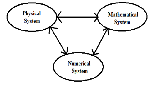
Fig. 3.1: Simple definition of modelling.
3.3.1 Properties of Mathematical Modelling – We prefer mathematical modelling because of the following reasons –
- With the help of mathematical model we can understand and investigate the meaning of equations and useful relations.
- It becomes very simple to make a educational environment in which preliminary person can be interactively occupied in guided inquiry and hands on actions with the help of mathematical modelling software (like – Stella II, Excel, online JAVA, MATLAB).
- Mathematical model is build up after the development of conceptual model of physical system. It is used to calculate approximately the quantitative presentation of the system.
- In order to spot a model’s strengths and weaknesses, quantitative outcomes obtained from mathematical modelling can be compared with observational information.
- The most important element of the resultant “complete model” of a system is mathematical model. Complete model is an assembly of theoretical, physical, numerical, visualization and statistical sub-models.
3.4 Types of Mathematical Modelling
These can also be divided into either numerical models and analytical models.
3.4.1 Numerical Modelling – It is one of the type of mathematical modelling in which numerical time stepping method is used to obtain model response over time. Results are presented in the form of graph or table. In this thesis numerical modelling is used to analysis the design characteristic of Bilayer Organics Solar Cell.

3.4.2 Analytical Modelling – Modelling having a closed form results is called analytical modelling. In closed form results, mathematical analytic functions are used to present the response to the equations that describe variation in a system.
3.5 Electrical Modelling
In this section, the electrical model for bilayer organic solar cell is described. One of the important characteristics of organic materials is their extremely small mobility, which makes modelling of their electrical properties difficult. Another problem in the electrical modelling of organic thin film devices (e. g. planar organic solar cells) was the lack of unique and precise electrical parameters for very thin layers of materials and occasionally lack of any information. Here with the aid of a self consistent loop between the Poisson equation and continuity equations for electrons and holes, the I-V curve of the device is calculated.
It is assumed that the electrical current is due to the drift-diffusion transport of carrier. Consequently, in order to model the drift diffusion equations, a self consistent loop between the solutions of Poisson’s equation and two separate continuity equations for electrons and holes is needed. The design of the loop should be in a way such that the solution of each equation can be used as the initial conditions for the others, to generate a self correcting mechanism.
The model that is used is based on the following assumptions:
- The generated excitons are separated right after absorption and the numbers of the generated electron-hole pairs are directly imported into the continuity equations as the generation rate .
- The transport properties of the organic materials can be totally modelled by mobility, DOS, bimolecular recombination term and doping levels.
- The connections between different layers follow the physical rules of hetero-junction connections between conventional semiconductors interfaces.
The other two equations, which are solved in a closed loop with the mentioned Poisson equation, are two separate continuity equations one for the electrons and one for the holes. The flowchart of the electrical model using the mentioned equations is shown in Fig. 3.2.
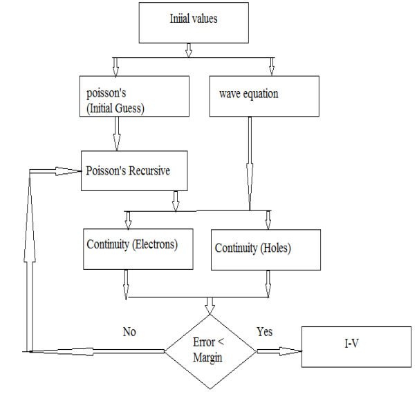
Fig. 3.2 : Flowchart of electrical model.
3.6 Work Done in Modelling and Simulation of OSC
Pettersson et al (1999)[8] have reported a model based on the experimental short circuit light generated current action spectrum of poly(3-(4’-(1”,4”,7”-trioxaoctyl)phenyl)thiophene) (PEOPT)/C60 fullerene hetero-junction photovoltaic devices. This modelling was completely based on the assumption that generation process of photocurrent is the result of creation, diffusion and dissociation of excitons. Using complex refractive indices and layer thickness, internal optical electric field was computed. We got values for exciton diffusion length of 4.7 and 7.7 nm for PEOPT &C60 respectively. Computed photocurrent and electric field distribution were used to study the effect of geometrical architecture with respect to the efficiency of device.
Cheknane et al (2007)[9] has reported a photovoltaic cell in which photo-active layer of MDMO-PPV and PCBM material is sandwiched between ITO and Al electrodes, there is an additional interfacial layer of PEDOT/PSS on the top of ITO. Comparision between V-I characteristics of device with and without extra interfacial layer is done and modelled by electrical equivalent circuit. Simulation results show that V-I characteristics of bulk hetero-junction solar cell is affected by extra interfacial layer of PEDOT/PSS.
Hwang et al (2007)[10] has reported drift-diffusion time dependent model of OSC based on blends of P3HT and red polyfluorene copolymer. In this model electron trapping and field dependent charge separation is used to investigate the device physics. This model is used to reproduce practical light-generated current transients observed in response to variable intensity step function excited light.
Vervisch et al (2011)[11] has reported OSCs simulation using finite element method. Using finite difference time domain process, optical modelling is done and electrical characteristics is obtained by solving Poisson’s and continuity equations. Simulation results show the effect of physical parameters like exciton lifetime on OSC performance.
Casalegno et al (2013)[12] has reported numerical approaches that give valuable information of microscopic processes underlying generation of photo-current in OSC. Here 3D master equation approach is used in which equations explaining particle dynamics rely on mean field guess and result is obtained numerically. Reliability of this method is tested against Kinetic Monte Carlo simulation method. V-I curve shows that the result of this method is very close to the exact result. Because of the adoption of mean field approximation for electrostatic interactions, we get biggest deviation in current densities. Strong energy disorder can also affect response quality. Simulation results show that master equation approach is faster than Kinetic Monte Carlo approach.
Foster et al (2013)[13] presented a drift-diffusion model to obtain V-I curves and equivalent circuit parameters of bilayer organic solar cell. Minority carrier densities are neglected and final equations are solved with internal boundary condition on material interface and ohmic boundary condition on contacts. From the solution of this model V-I curves are calculated.
3.7 Introduction to MATLAB
MATLAB [13] is a high performance language for technical computing. It integrates calculation, visualization and programming in a simple to use surroundings where troubles and solutions are presented in well-known mathematical notation. MATLAB can solve technical computing troubles faster than conventional programming language (like – Forton, C, C++). Typical uses include –
- Financial modeling and investigation
- Computational biology
- Math and computation algorithm development
- Data acquisition modeling
- Simulation and prototyping data study
- Exploration and visualization
- Graphics application development for scientific and engineering field
- Graphical user interface building
Matrix laboratory is the full form of MATLAB. Basic data element in MATLAB is an array which does not need dimensioning. With the help of MATLAB number of technical computing troubles mainly those with vector and matrix formulations can be solved in a fraction of time. Basically it was written to give simple access to matrix software. For advance science, mathematics, engineering field and high productivity industrial research, progress and study MATLAB is very important instruction tool. Comprehensive collection of MATLAB functions are toolbox. Toolboxes of MATLAB permit us to study and apply specific technology. Toolboxes are available in different areas like – neural network, communication, signal processing, fuzzy logic, simulation, control system and many others.
Differential equations are solved very easily in MATLAB [14-17]. We can also do modeling and simulation of solar cell using MATLAB [18,19].
3.8 Conclusions
This chapter explains about modelling and simulation. Presentation of physical configuration or activities of device by conceptual mathematical model that approximates this behavior, is called modeling. Model may either be closed form equation or arrangement of simultaneous equations that are numerically solved. Analytical and numerical both type of analysis can be used in modeling. Simulation is process of imitating the physical system behavior by considering the characteristic of an analogous but different system without resorting direct practical experimentation. For simulation we are using MATLAB which is a high performance technical computing language. We get that MATLAB integrates calculation, programming and visualization in a simple to use surroundings where mathematical expressions are used to express troubles and solutions.
Because of all these qualities of MATLAB a system of number of numerical equations used for electrical modelling of bilayer organic solar cell are solved easily and in better way as compared to other programming languages.
3.9 References
[1] B. P. Zeigler, Wiley, New York, (1976).
[2] A. M. Law and W.D. Kelton, 2nd ed., McGraw-Hill, New York, (1991).
[3] F. Haddix, Paper 01F-SIW-098, Proceedings of the Simulation Interoperability Workshop, Fall (2001).
[4] A. Crespo-Márquez, R. R. Usano and R. D. Aznar, Proceedings of International System Dynamics Conference, Cancun, Mexico, The System Dynamics Society, (1993), 58.
[5] J. S. Kumari and C. S. Babu, International Journal of Electrical and Computer Engineering (IJECE), 2(1), (2012), 26-34.
[6] P. Sudeepika, G.Md. G. Khan, International Journal of Advanced Research in Electrical,Electronics and Instrumentation Engineering, 3(3), (2014), 7823-7829.
[7] M. Abdulkadir, A. S. Samosir, A. H. M. Yatim, International Journal of Power Electronics and Drive System (IJPEDS), 3(2), (2013), 185-192.
[7] L. A. A. Pettersson, L. S. Roman, and O. Ingana, Journal of Applied Physics, 86, (1999), 487-496.
[8] A. Cheknane, T. Aernouts, M. M. Boudia, ICRESD-07, (2007), 83 – 90.
[9] I. Hwang, C. R. M. Neill, and N. C. Greenham, Journal of Applied Physics, 106, (2009), 094506:1-10.
[10] W. Vervisch, S. Biondo, G. Rivière, D. Duché, L. Escoubas, P. Torchio, J. J. Simon, and J. L. Rouzo, Applied Physics Letters, 98, (2011), 253306:1-3.
[11] M. Casalegno, A. Bernardi, G. Raos, J. Chem. Phys., 139(2), (2013).
[12] J. M. Foster, J. Kirkpatrick, and G. Richardson, Journal of Applied Physics, 114, (2013), 104501:1-15.
[13] A. Knight, CRC Press LLC, (2000).
[14] R. K. Maddalli , Indian Journal of Computer Science and Engineering, 3(3), (2012), 406-10.
[15] Z. M. Kazimovich and S. Guvercin, International Journal of Computer Applications, 41(8), (2012), 1-5.
[16] A. B. Kisabo, A. C. Osheku, A. M. Adetoro, A. Lanre and A. Funmilayo, International Journal of Scientific and Engineering Research, 3(8), (2012), 1-7.
[17] V. Nehra, I.J. Intelligent Systems and Applications, 05, (2014), 1-24.
[18] S. Nema, R. K. Nema, and G. Agnihotri, International Journal of Energy and Environment, 1(3), (2010), 487500.
[19] M. Edouard, D. Njomo, International Journal of Emerging Technology and Advanced Engineering, 3(9), (2013), 24-32.
Cite This Work
To export a reference to this article please select a referencing stye below:
Related Services
View all


DMCA / Removal Request
If you are the original writer of this essay and no longer wish to have your work published on UKEssays.com then please click the following link to email our support team:
Request essay removal